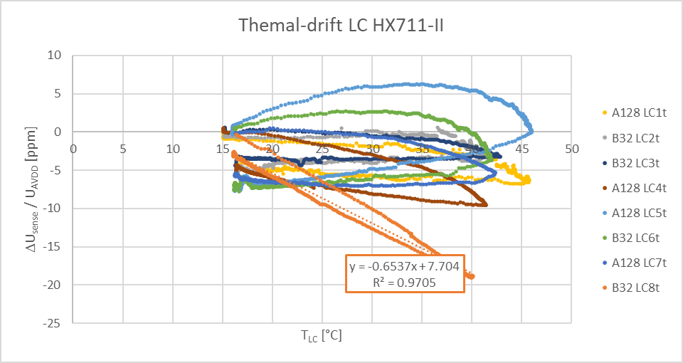
Sometimes, simpler is better. Here is a new version of load cell temperature compensation, which is simpler and works better. All the beginning is the same (the model is unchanged), only the way the model is applied is different. Also I collected a new set of data with more precise temperature measurement to better test the model. The result appear on the last chart; it show that weight measurement drift with temperature can be almost completely eliminated.
In case M. Moderator reads this, can you please remove the previous post (I am repeating everything here below)) ? It would make the thing easier and quicker to grab for new comers interested in this topic. [M. Moderator @wtf: You are reading the updated version from April, 11th 2022, right here!]
Here is the new post, with complete explanation:
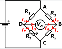
The weight sensor is a strain gauge, which is a resistor which value varies very slightly when the metal in which it is embedded deforms under the effect of the weight to be measured. This resistor forms with 3 other fixed resistors of known values a Wheatstone bridge. The circuit to which the strain gauge is connected measures the voltage difference VG and then a simple calculation gives the resistance RX of the strain gauge.
When no load is put on the scale, the readout of the ADC is called the offset.
The output of the ADC when a load is applied to the scale represents the value of that mass, plus the offset.
Therefore, in order to measure a mass, we measure the output of the ADC when the mass is applied on the scale, from which we subtract the offset and the result is divided by a fixed factor representing how much the ADC value varies for 1 g of load. Load cells providers state that their products are “temperature compensated”, which means that this difference (value read when load is applied minus value read when no load is applied) is a more or less independent of temperature. But the value of the offset itself IS temperature dependent. According to my measurements, it varies linearly with the temperature with a slope depending on the load cell. I tested six different H40 load cells from the German supplier Bosche (by far the best supplier I have tested) and I was able to measure slopes that varied from 1 to 7g per degree. When the temperature fluctuates 20 degrees, the best loadcell drifts by 20 g, which seems acceptable and probably does not require implementing temperature compensation. On the other hand, the worst one drifts by 140 g for this temperature range, justifying a temperature compensation.
We will see in this document how to implement an efficient temperature compensation based on a proposed modeling of the loadcell and corresponding mathematical calculations.
At the end this document, we will apply the proposed temperature compensation formulas to actual data collected on a beehive scale and will show that temperature drifts can be almost entirely compensated thanks to the proposed model.
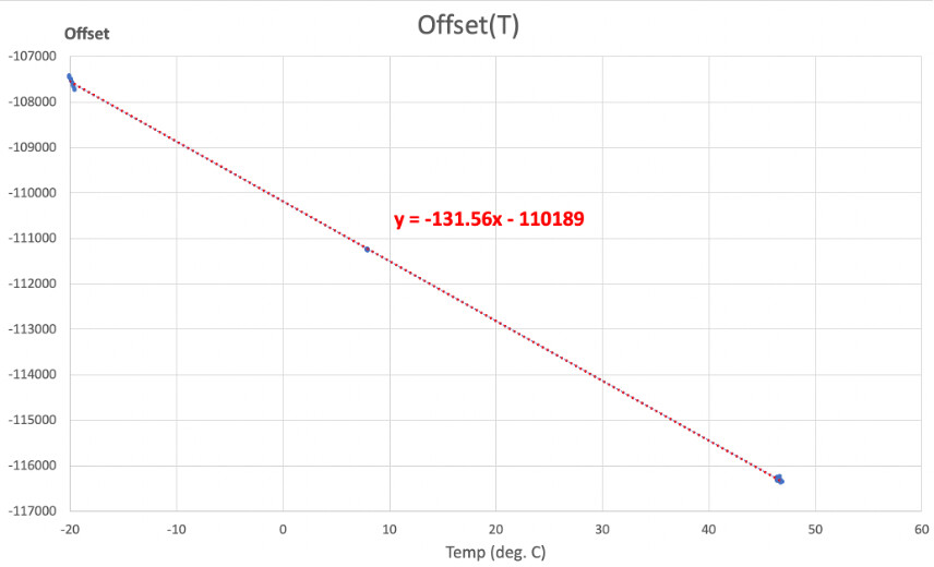
The graph above shows the variation of the offset measurement as a function of temperature for an “average” load cell among the six that I have tested. In this particular case, 45 units correspond to 1 g so the offset varies 2.85 g per degree.
On a “normal” scale, the variation of the offset with the temperature does not pose a problem because offset is measured each time power is switched on; the value of the mass minus the offset is therefore independent of the temperature. But “zero-ing” the offset at each measure is not possible with a hive scale because the mass is applied permanently and the value of the offset that is subtracted from the measurement is an offset measured beforehand at a temperature different from the actual measurement temperature. .
If the load cell is calibrated beforehand and we know how the offset varies with temperature (linear curve here above), we should be able to correct the measurement by calculating the true offset at the current temperature instead of the one measured beforehand at a different temperature. Unfortunately the load cell has a certain thermal inertia and when the outside temperature varies, the temperature of the load cell does not vary by the same value. We must therefore find a way to determine what is the internal temperature of the load cell based on historical temperatures.
The load cell, especially when fixed in its scale structure, has a certain heat capacity C. Its temperature, which is assumed to be homogeneous inside the load cell, does not vary in the same way as the outside temperature because the load cell mounted in the scale has a given thermal conductivity σ which is not infinite. The quantity of heat dq that is absorbed by the load cell during a time dt causes its temperature to change by ![]() and it’s easy to understand that the higher the temperature difference between the load cell
and it’s easy to understand that the higher the temperature difference between the load cell ![]() and the outside temperature
and the outside temperature ![]() the faster the load cell temperature changes.
the faster the load cell temperature changes.
For an electronics engineer, all of this reminds what happens when a capacitor is charged through a resistor from a constant voltage source.
And as expected, when a temperature step is applied to the load cell mounted in the scale, we can observe that the ADC output evolves over time with a curve that looks a lot like the charge of a capacitor C (here the heat capacity of the scale) at constant voltage (here the temperature step ∆T) through a resistor (homogeneous with the inverse of the thermal conductivity: 1/σ ).
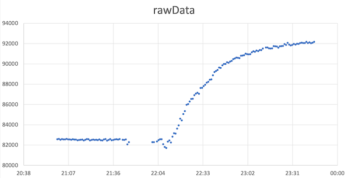
The graph above shows the change in ADC output when the unloaded scale is moved from an indoor environment with a stabilized temperature of 21°C to an outdoor environment with a temperature of -1°C (almost) stable over the duration of the measurement.
We now need to put all that in equations…
In the analogy with the evolution of the voltage U measured on a capacitor C when it is charged at constant voltage E through a resistor R , the diagram is as follows:
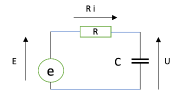
The charging current i is equal to the amount of energy stored by the capacitor per unit of time, i.e. i=dq/dt and therefore, knowing that U=qC the current is ![]()
We can therefore express the voltage E as follows:
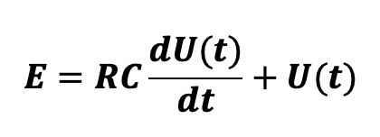
In our case, R is homogeneous with 1/σ , the inverse of the conductivity, E is homogeneous with the variation of the offset resulting from the temperature step if the conductivity were infinite (let us call ![]() this offset value), C is homogeneous with the heat capacity of the load cell and U is homogeneous with the actual measured offset O(t). The differential equation which defines the temperature is therefore:
this offset value), C is homogeneous with the heat capacity of the load cell and U is homogeneous with the actual measured offset O(t). The differential equation which defines the temperature is therefore:
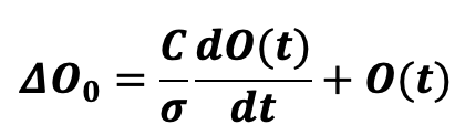
O(t) being the offset increment since the temperature step was applied
It can be demonstrated in mathematics that the solutions ![]() of a differential equation of order 1 with constant second member, of type
of a differential equation of order 1 with constant second member, of type ![]() are of the form:
are of the form:
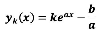
k being a real number that is determined in physics with the initial conditions. In our case, the differential equation can be written:
![]()
So we have :
And the solutions to our differential equation are therefore of the form:
![]()
We know that at time t=0, the increment of the offset is zero and we can therefore deduct that
![]()
And therefore, the offset increment since the time the temperature step was applied is calculated as follows:
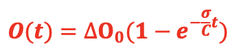
The time constant σ/C is unknown; we will therefore determine it graphically by representing on the previous graph the equation obtained above. We see on the graph below that with a time constant equal to 17 (the time being counted in minutes), the two curves overlap almost perfectly, which seems to indicate that the chosen model is correct.
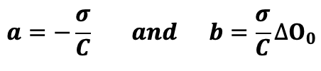
By the way, offset being proportional to weight, the previous equation can also be written as:
Which means – it’s important to be precise because the notation is a bit misleading – that when a temperature step corresponding to a weight readout change of ![]() (after an infinite time) is applied, the actual readout of the weight is evolving over time according to the above equation, knowing of course that the weight itself is stable over time.
(after an infinite time) is applied, the actual readout of the weight is evolving over time according to the above equation, knowing of course that the weight itself is stable over time.
But we are not done yet. The experiment and the calculations that we have just made have allowed us on one hand to verify that the chosen model is correct and on the other hand to determine graphically what is the time constant of the scale measurement process, but we still do not know not how to calculate the temperature of the load cell based on the outside temperature, which of course is varying over time instead of being constant as in our experience…
Here we need to make an approximation and we will assume that the temperature evolution over time is a series of small temperature steps applied each time we take a weight measure. In others terms, if we take a measure every 15mn, we will assume that the load cell temperature when we take a measure is resulting from :
-
a temperature step applied 15 minutes ago and equal to the temperature difference between current measure and previous one
-
another temperature step applied 30mn ago and equal to the temperature difference between the measure we took 15mn ago and the one we took 30mn ago
-
plus the one before, etc, etc…
Because we know the time constant is 17mn, we will consider only the last 5 measures – which means that anything that happened before 75mn ago is ignored.
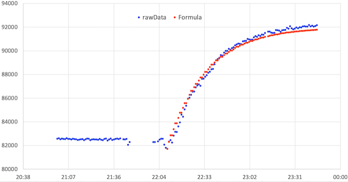
In order to test this model, we have put the scale in a closed box (to make sure temperature is correctly measured, avoiding the effect of sun shining on the scale) with a ~2Kg weight on it and we put this box outside during a week. Then we collected the raw weight measurement every 15mn along with the temperature at the same time.
Here is the corresponding chart:
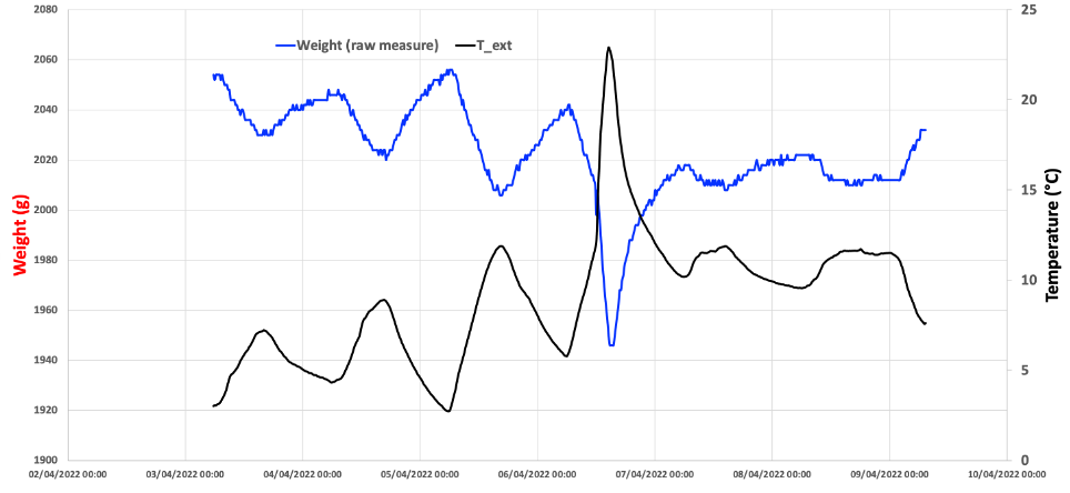
The weight measurement when a constant mass is applied on the scale does varies quite a lot with temperature. We have seen before that weight readout is proportional to temperature and by looking at the extremes points of the above graph, we can calculate what is the slope α of corresponding linear curve
![]()
In this case, ![]()
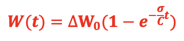
So when a temperature step ![]() is applied on the scale, the weight measurement changes – after an infinite time where temperature stays constant – by a value
is applied on the scale, the weight measurement changes – after an infinite time where temperature stays constant – by a value ![]()
The previous equation can therefore be written ![]()
So each time we take a new measure, we applied this formula with t=15mn, ![]() being the temperature difference between this measure and the previous one, 15mn ago. This is giving us the value by which the weight measurement has changed as a result of this temperature step. To this value we add the weight measurement change resulting of the temperature step applied 30mn ago (t=30), plus the one 45mn ago, plus the one applied 60mn ago plus the one applied 75mn ago and we stop here because further in the past, the effect of a temperature step vanishes almost entirely.
being the temperature difference between this measure and the previous one, 15mn ago. This is giving us the value by which the weight measurement has changed as a result of this temperature step. To this value we add the weight measurement change resulting of the temperature step applied 30mn ago (t=30), plus the one 45mn ago, plus the one applied 60mn ago plus the one applied 75mn ago and we stop here because further in the past, the effect of a temperature step vanishes almost entirely.
The process is therefore the following: each time a weight measurement is taken, the above process is applied and the calculated weight measurement change is subtracted from the measured weight, giving a temperature compensated weight measurement.
The graph here below is the same as the previous one, on which the red curve representing the temperature compensated weight is shown. This weight is staying relatively flat when temperature changes, which seems to indicate that the model and the way it is applied is working OK.
The glitch in the middle corresponds to a move of the box in which the scale was placed from shadow to sun (as indicated by the sudden temperature increase). It’s likely that this move has induced some false measurement.
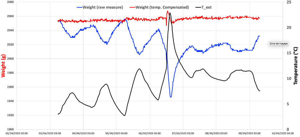
Apart from the glitch resulting from a move of the scale, we now have a weight measurement system that is largely immune to temperature changes.
Practically, the key to have a good measurement is to make sure the temperature is correctly measured, which is not as simple as it seems especially when sun is shining (as soon as sun shines directly on either the load cell or on the temperature sensor, it creates bad measures; and if it shines on the cable bringing the load cell signal to the ADC, it creates another perturbation - called Seebeck effect - that is well explained by @weef in this post).